
LiDAR Analysis
@ NIST
-
Evaluate the accuracy of LiDAR-based object detection in 3D environments.
Segment objects of interest from point cloud data using a computer vision routine.
Calculate average distances from segmented points to predicted object surfaces to assess alignment.
Quantify how well raw LiDAR data conforms to expected geometries in robotics applications.
-
Summer Research Fellow
-
May-Aug 2025
-
Python for planar regression, figure creation, and systematic file renaming. Libraries used:
Plotly
Scikit-learn
Numpy
Matlab for Principal Component Analysis and figure creation.
Unix and Powershell for SDK installation.
-
While specific outcomes are awaiting review, the script procedure was successful in revealing performance of various LiDAR sensors.
Quantified flatness deviation across test surfaces, validating PCA-based plane fitting as a reliable ground truth method.
The National Institute of Standards and Technology (NIST), an agency under the U.S. Department of Commerce, promotes innovation and industrial competitiveness. In support of this mission, my work focuses on characterizing the performance of various LiDAR systems and developing standardized testing procedures to lower the barrier to entry for companies entering the robotics industry.
Background
LiDAR (Light Detection and Ranging) is an active sensing technology that emits pulses of light and measures the time it takes for each pulse to reflect off a surface and return to the sensor. Given the constant speed of light, this time-of-flight measurement can be used to calculate distance and generate a three-dimensional point cloud representing the environment.


methodology
Figure 1: Illustration of the test setup with accounts for beam divergence
Setup
By positioning a 50% Lambertian target within the sensor's field of view, we can establish a reference plane across the target's surface and measure the average distance between individual data points and this plane as our noise metric.
two independent variables were controlled:
Target distance
Incident angle (angle between the plane’s normal vector and the incident ray)
LiDAR beams widen with distance due to natural divergence. When part of the beam misses the target, it causes backscattering and data distortion, requiring the measurement plane to be cropped to the beam dimensions.
The beam cross-section becomes elliptical at steep incident angles, with the major axis extending further across the surface, necessitating wider cropping areas for accurate measurements.
PCA
Applied Principal Component Analysis (PCA) for plane fitting in 3D point cloud data, enabling surface characterization independent of target orientation.
PCA decomposes the data by:
Computing the covariance matrix of the point cloud.
Extracting eigenvectors (principal components) and eigenvalues (variance explained).
Ranking vectors by their corresponding eigenvalues to identify directions of greatest variance.
In 3D:
The first two principal components span the plane of best fit.
The third principal component, with the lowest variance, serves as the surface normal vector.
Constructed a local 2D coordinate system aligned with the target surface for cropping:
New x-axis: Cross product of
[0 0 1]and the surface normal vector.New y-axis: Cross product of the normal vector and the new x-axis.
This basis allows cropping to match the incidence angle and target distance.
2D beam cropping is now possible with this new coordinate system.
Because rotating LiDARs use a rotating vertical beam array, the resulting point cloud forms a vertical stack of rings. To ensure a valid planar regression, at least two vertical rings are needed. Therefore, PCA eigenvalues are used to verify that vertical variance is not significantly lower than horizontal, confirming that the data spans a full 2D surface rather than a single arc.

Figure 2: PCA-aligned coordinate system with Basis Vectors 1 and 2 spanning the target plane. Colors show point cloud residuals relative to the best-fit plane.
Cropping results
Before cropping:
Residuals increased significantly with planar distance from the centroid.
Indicated edge effects and misalignment in the regression region.
After cropping using the local PCA-aligned frame:
Residuals became roughly uniform across the target surface.
Demonstrated effective removal of outlier geometry and improved planar fit accuracy.
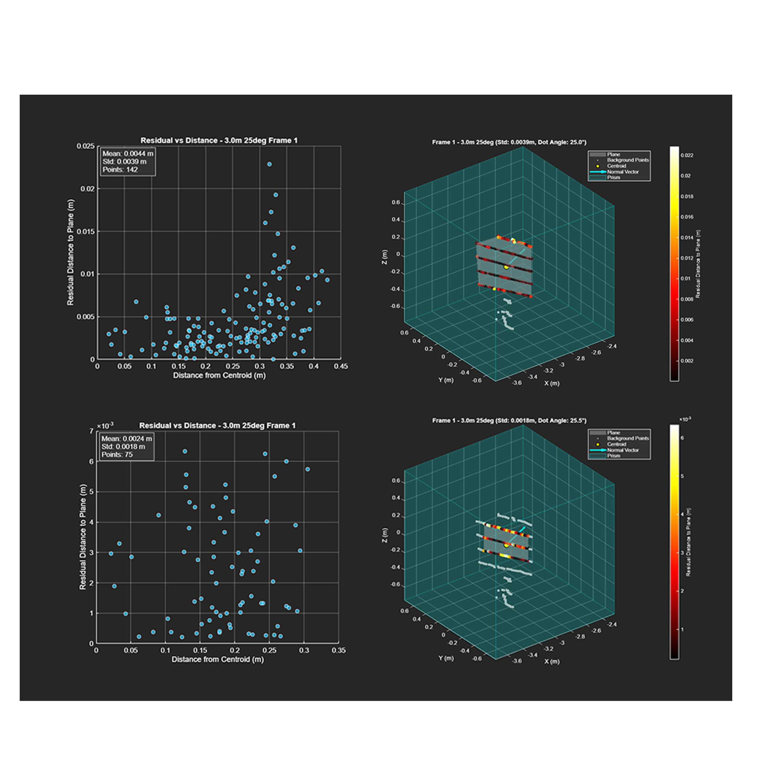
Figure 3. The top panels show residuals versus distance along with the original point cloud prior to cropping, while the bottom panels show the same plots after cropping, highlighting the improved fit and reduced residuals.
script procedure
Data Collection:
After configuring and connecting the sensor, 200 frames are recorded for each combination of:
Distance: 3 m to 11 m
Incident angle: −15° to 75° in 10° increments
File Renaming (Python):
A Python script renames all.pcapand.jsonfiles using the format:
"<distance>m_<angle>deg.<pcap/json>"Processing (MATLAB, Python for some sensors):
Each frame is processed individually:A 3 m-wide rectangular prism is centered at the specified distance along the
[1 0 0]vector.PCA is performed to fit a plane and compute residuals.
A scatterplot of residuals is generated for all frames.
A .xlx file of statistics for each frame is output.
User Interaction:
The script prompts the user to input:Distance, angle, and frame number
Whether to visualize the entire scan or just the cropped region.

Figure 4: Uncropped visualization of a LiDAR frame showing background points, the regression plane, centroid, normal vector, and bounding prism.